Video Physics: Ping-Pong Ball Drop

In which I'm back on my bullshit...

Feb 20, 2025

Tuesday’s post about structure in education was useful as a head-clearing exercise, but didn’t exactly move my class prep forward. The same process of noodling around with ideas for next term’s advanced lab course prompted me to go down in the lab and fool around with video physics again, though, which is a much more positive development along multiple axes.

As noted on Tuesday, one of the things we’re doing next term is adding a more structured first lab to introduce students to using Tracker Video with an eye toward having them do their own video-analysis projects at the end of the term. We did the final project part last year with kind of mixed results because they didn’t really grasp the software well enough from just reading the documentation. (This led to a whole series of blog posts over the summer where I re-did video analysis projects that hadn’t quite worked…)

The idea is to give them a step-by-step intro to Tracker using a canned video (having them determine the acceleration of gravity from a clip of me dropping a baseball), to learn how the basic features work. Then we’ll ask them to make their own videos of some relatively straightforward phenomenon with an answer that’s less well known, and do the analysis of that.

My first thought was to simply ask them to do video analysis of the coffee filter drop lab, which most of them did in intro mechanics their first year, in a less sophisticated form (just using a stopwatch to determine the terminal speed for different masses). That has some slightly tricky aspects, though, as noted toward the end of that post— the filters tend to flutter slightly, changing the apparent shape, which can confuse the autotracker. A more stable shape might work better, in terms of the video quality, and thus might allow for more satisfying quantitative results. But how to do this?

The first issue is finding something with a more visually consistent shape that would show a significant effect of drag, whose mass could be varied. The obvious shape for this purpose is a sphere, and, indeed, we have a wide variety of small balls around the department, but most of them are a little too heavy for air resistance to really matter. In the process of poking around looking for something else, though, I was reminded that I have a bunch of ping-pong balls that were used for some demo. A quick test video confirmed that a ping-pong ball in fact falls notably slower than one of the solid plastic balls we use in the Pasco projectile launchers for intro labs. Of course, they’re dramatically different sizes, which kind of undermines any attempt to do anything quantitative relative to the drag force….

However… A ping-pong ball is very light (about 2.1 grams) because it’s made of very thin plastic. So I made a trip to the Biology department and found a syringe (thanks, Amy!) that I could use to make a tiny hole in the ball and fill it with about 25cc of water. That gave me a way to get two spheres of exact same size with dramatically different masses (the water-filled one was around 26 grams). And, indeed, dropping a weighted ping-pong ball looks distinctly different than dropping a hollow one:

That’s a graph of position vs time extracted from the video, clearly showing a more rapid acceleration for the heavy ball than the light one. We can do the same thing with the velocity vs time:

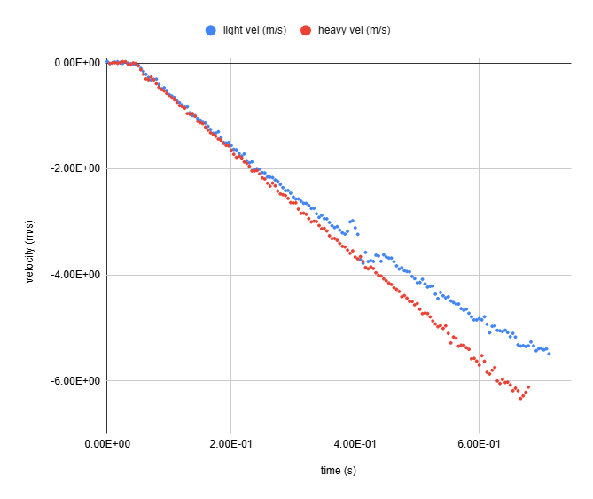
This shows the instant of the drop much more clearly (this uses a dummy time scale and I matched the two series up by eye, and you can also see that the track for the light ball is curving upward. That’s exactly what you expect: the drag force should increase like the square of the speed, getting dramatically bigger as the ball falls. That leads to a slope that’s shallower for the light ball, and gets more so over time— if it fell far enough to reach terminal speed, the line would go completely flat.

So, qualitatively this is doing the right thing. But the question I went into this with was whether we can do anything quantitative with this system— extracting some kind of number that could be compared to an expected value or theoretical prediction of some kind. The only plausible choice here would be to see if we could extract a drag coefficient, the quasi-empirical number that accounts for the geometry of an object subject to drag in air.

This requires measuring a force, which we can get from the acceleration, but there we hit a problem: as you can see from the graph, the velocity data is somewhat noisy, and a little bit of noise in the velocity measurements turns into a lot of noise in acceleration measurements. This can sorta-kinda be addressed by using a larger number of points, at the cost of losing some time resolution.

I attempted a really coarse version of this, by looking at the first twenty data points after the drop, and the last twenty before the ball hit the floor, and fitting slopes to those to find the acceleration, which you can see in this kind of busy graph:

Again, qualitatively, this is great: At the start of the drop, the light and heavy ball have almost exactly the same acceleration (10 m/s/s and 10.4 m/s/s, respectively; a little higher than the textbook value, but I didn’t calibrate the clip all that carefully), because the air drag is negligible. At the end of the clip, the heavy ball is both moving faster and accelerating faster (8.2 m/s/s vs. 5.3 m/s/s)1, as you would expect, since the drag force pushing up depends on speed but the gravitational force pulling down depends on mass.

Does this work out quantitatively? I initially thought not, but I was making a very dumb error2, and when corrected, it’s surprisingly good! I can use the difference between early and late accelerations to find the drag force for the light ball, and then convert that to a drag coefficient using the dimensions of the ping-pong ball and the standard density of air. The value I get from that is 0.499, which is right smack in the range of what you find quoted as the value for a sphere.

How reliable is this? That, unfortunately, is kind of hard to say— it’s entirely possible that this nice agreement is just a happy accident. If I do the same analysis for the heavy ball (excluding the couple of weird points mentioned in the footnote), I get a coefficient of around 0.8 which is way too big. A similar analysis on a different clip (which wasn’t as good, video-wise) comes out with a “drag coefficient” of 0.26. The heavy ball in that clip barely changes acceleration from early to late, so you would infer a coefficient of near zero, which can’t really be right, either. On the other hand, the third clip I have (from the very first demo run) comes out at 0.44, but uses a different brand of ping-pong ball whose mass and dimensions I didn’t check. The upshot of which is: it’s probably fairly good?

So, is this a useful lab? It’s tough to say. On the one hand, it’s less of a repeat than doing the coffee filters, and the video analysis piece is much more straightforward. Not perfectly— you can see a weird glitch in the middle of the velocity-time graph that I don’t really understand— but tracking the fall of a round thing is much less demanding on the software, and that somewhat simplifies the analysis stage. Getting a quantitative result you could compare to a “known” value is a nice bonus— our students are weirdly fond of calculating “percent difference”…

On the other hand, though, the effect is much more dramatic in the coffee filters, small stacks of which do manage to reach terminal speed. You can’t do any quantitative comparison— I have no idea what the drag coefficient of a coffee filter “should” be— but then, that avoids the angst that comes out when quirks of the fitting end up giving numbers that are wildly different than the expected values.

I suspect the “right” answer here may be to just do the coffee filter thing as the first lab exercise next term, since it’s familiar and relatively reliable, and keep the ping-pong ball thing in mind as a potential project to suggest to a student who has trouble coming up with a good idea of their own. There are some straightforward extensions— measuring the effect for several different masses (not just “completely full” and “completely empty”), using a different pair of objects (a colleague suggested comparing a real golf ball to an indoor practice golf ball), or just letting them fall farther so there’s a bigger acceleration difference (which I didn’t attempt because that would require finding some way to get a relatively uniform background to shoot against, which is tricky in our building)— that could make this a nice project.

Or it may just turn out to be a way for me to entertain myself for a week or so this summer… Even if nothing comes of it, it kept me from looking at news or social media for several hours yesterday, and that’s a Very Good Thing these days.

If you want to see whether I do anything else with this, here’s a button:

And if you have suggestions of related things I ought to try, or spot any errors in my approach, the comments will be open:

Counting Atoms

Discussion about this post